Multivariable Calculus

We consider functions from \(\mathbb{R}^n\) to \(\mathbb{R}^m\) which are expressed as

\[\mathbf{f}(\mathbf{x})=\mathbf{f}(x_1,\cdots,x_n)=(f_1(\mathbf{x}),\cdots,f_m(\mathbf{x}))\]

Different Forms of Multivariable Functions

Parametric Surface

Note

• If \(n=1\) and \(m > 1\) then the functions \(f:\mathbb{R}\mapsto\mathbb{R}^m\) are known as parametric sufraces.

• Example: \(f(x)=(x, x^2)\)

Scalar field

Note

• If \(n> 1\) and \(m=1\) then the functions \(f:\mathbb{R}^n\mapsto\mathbb{R}\) are known as scalar fields.

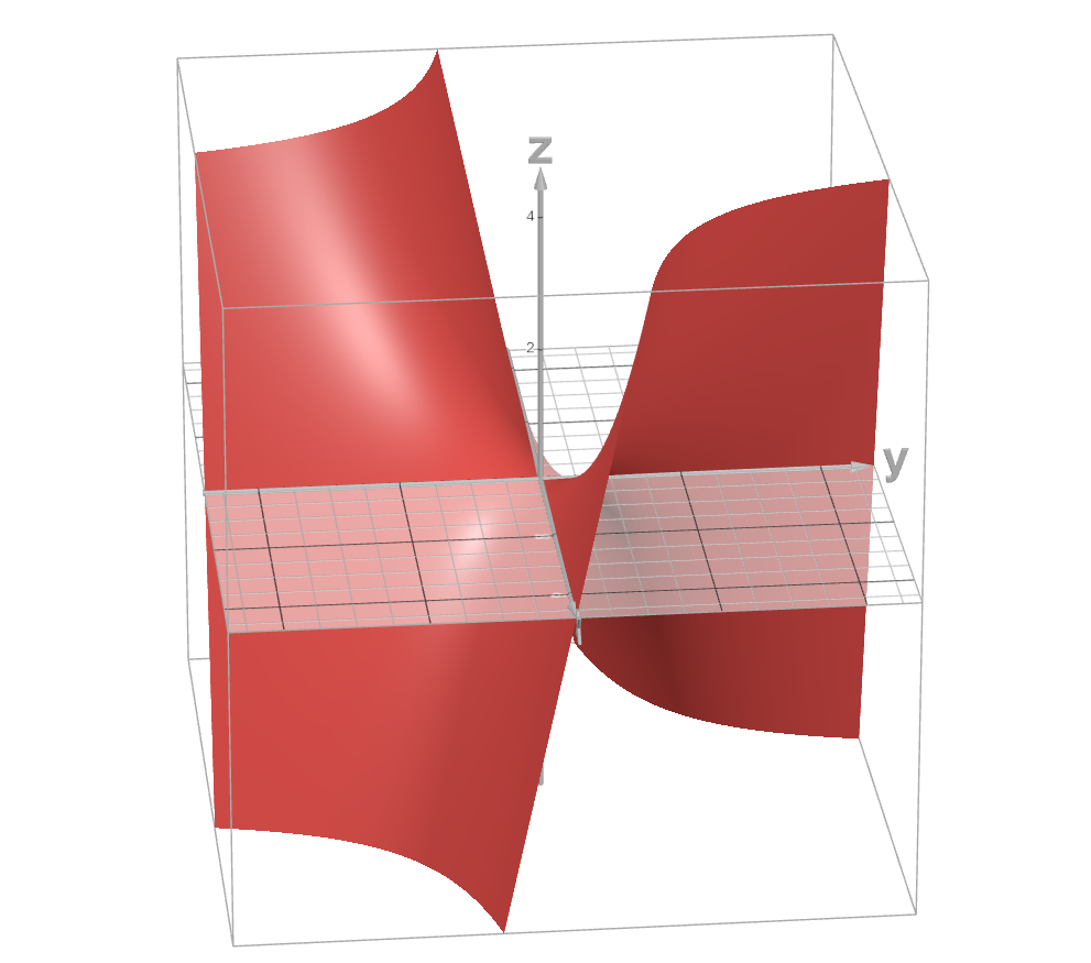
• Example: \(f(x,y)=xy\)

Vector field

Note

• If \(n> 1\) and \(m> 1\) then the functions \(\mathbf{f}:\mathbb{R}^n\mapsto\mathbb{R}^m\) are known as vector fields.

• Example: \(f(x,y)=(x^2,\sin(y),x+y)\)

Continuity

Note

• We have a function \(\mathbf{f}\), from an open set \(E\in\mathbb{R}^n\) into \(\mathbb{R}^m\).

• A function is continuous at a point if each of its components, \(f_k(\mathbf{x})\) is continuous at that point.

Differentiation

Directional Derivative as a rate of change in scalar fields

We have a function \(f\), from an open set \(E\in\mathbb{R}^n\) into \(\mathbb{R}\). We want to find a proper definition of derivative of \(f\) at some point \(\mathbf{x}\in E\).

Note

• There is a single direction along which we can approach a point \(x\in\mathbb{R}\).

• However, there are infinite directions along which we can approach a point \(\mathbf{x}\in\mathbb{R}^n\).

• Along each such direction, the rate-of-change in the function can be different.

• In order to apply the notion of single variable derivative, we can therefore reduce the function to a single dimensional one by looking at the slice along a particular line.

• We fix our direction along some vector \(\mathbf{u}\in\mathbb{R}^n\) and look at the rate-of-change of the function along \(\mathbf{u}\) as we move closer to \(\mathbf{x}\).

• For some \(h> 0\), we assume an open-ball around \(\mathbf{x}\) of radius \(h\cdot||\mathbf{u}||\), and define the ratio

  \[\frac{f(\mathbf{x}+h\cdot\mathbf{u})-f(\mathbf{x})}{h}\]

• We define a version of derivative as \(f'(\mathbf{x}; \mathbf{u})=\lim\limits_{h\to 0}\frac{f(\mathbf{x}+h\cdot\mathbf{u})-f(\mathbf{x})}{h}\)

Attention

We note that the open ball in this case is essentially an equivalent of an one dimensional interval.

Note

• If \(\mathbf{u}\) happens to a unit-vector, then our open ball is \(B_h(\mathbf{x})\).

• In this case, \(f'(\mathbf{x}; \mathbf{u})\) is called the directional derivative along \(\mathbf{u}\).

Partial Derivative

Note

• If the unit vector in a directional derivative is along any of the coordinate-axes, such as \(\mathbf{e}_k\), the directional derivative is called a partial derivative.

• Notation: \(D_k f(\mathbf{x})=f'(\mathbf{x}; \mathbf{e}_k)=\frac{\mathop{\partial}}{\mathop{\partial x_k}}f(\mathbf{x})\)

Directional Derivative isn’t sufficient

Warning

• A nice property of derivatives for single variable case is that if it exists at a given point, it implies that the function is continuous at that particular point.

• HOWEVER, existence of direcitional derivatives doesn’t imply continuity.

Example

See also

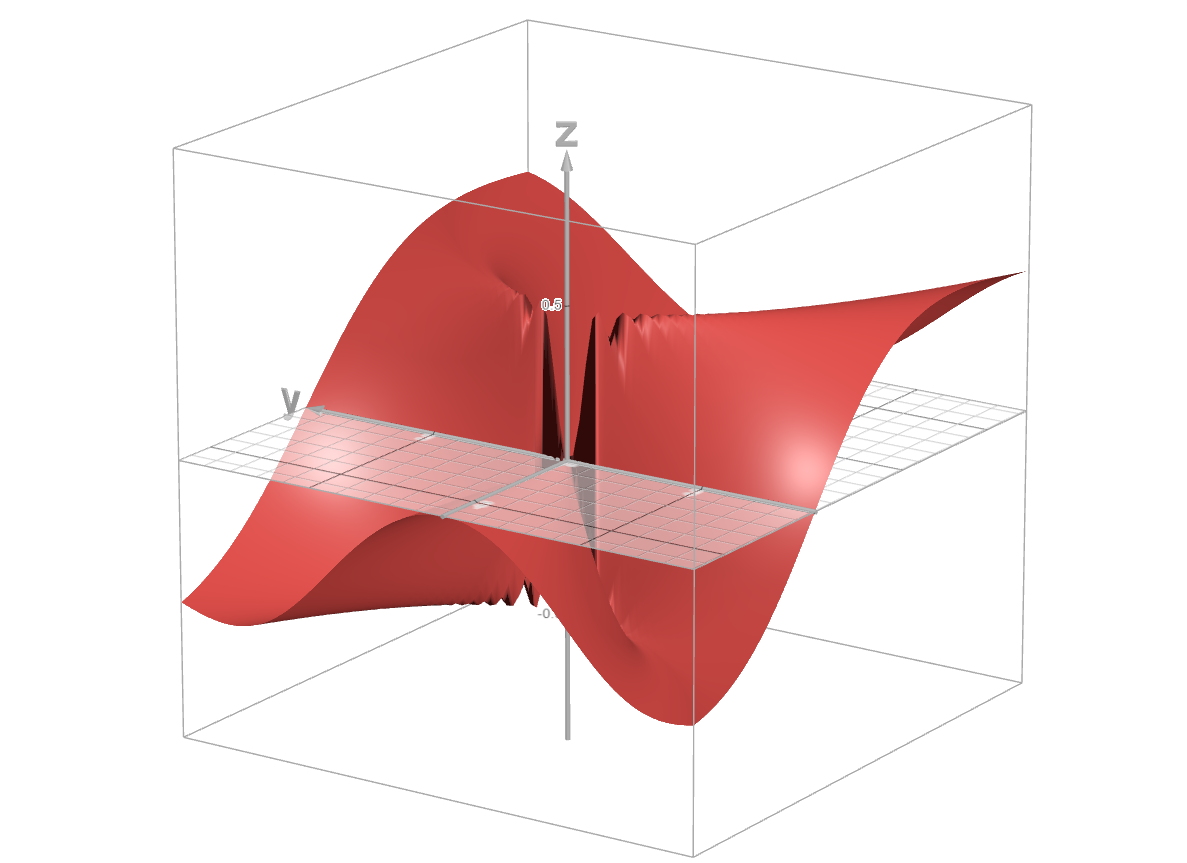
• We consider a scalar field

  \[\begin{split}f(x,y)=\begin{cases}\frac{xy^2}{x^2+y^4} & x\neq 0\\0 & x=0\end{cases}\end{split}\]

• We consider any arbitrary vector \(\mathbf{u}=(u_x,u_y)\) where \(u_x\neq 0\) and consider \(f'(x,y;\mathbf{u})\) at \(\mathbf{0}\).

  \[\frac{f(\mathbf{0}+h\mathbf{u})-f(\mathbf{0})}{h}=\frac{f(h\mathbf{u})}{h}=\frac{f(hu_x,hu_y)}{h}=\frac{hu_x(hu_y)^2}{h((hu_x)^2+(hu_y)^4)}=\frac{u_xu_y^2}{u_x^2+h^2u_y^4}\]

• Therefore, \(f'(x,y;\mathbf{u})=\lim\limits_{h\to 0}\frac{u_xu_y^2}{u_x^2+h^2u_y^4}=\frac{u_y^2}{u_x}\) which exists for all such \(\mathbf{u}\).

• We now consider another vector \(\mathbf{v}=(0,v_y)\) and consider \(f'(x,y;\mathbf{v})\) at \(\mathbf{0}\).

  \[\frac{f(\mathbf{0}+h\mathbf{v})-f(\mathbf{0})}{h}=\frac{f(h\mathbf{v})}{h}=\frac{f(0,hv_y)}{h}=0\]

• Therefore, a directional derivative exists along every conceivable direction.

Warning

• However, we note that along the parabolic path \(x=y^2\), \(f(x,y)=\frac{1}{2}\).

• This means that if we move along this parabolic path, the value of the function jumps from \(\frac{1}{2}\) to 0 at the origin all of a sudden.

• No directional derivative along any straight line can catch this jump, as along that line, we can always form tiny open balls which excludes the points in the parabola.

• Therefore, directional, and by extension, partial derivatives don’t define a proper differentiation.

Total Derivative as a linear approximation in general

We define the total derivative as a linear approximation of the function at close proximity of \(\mathbf{x}\).

Note

• Instead of checking from a single direction, we need to consider all directions at once.

• Therefore, we consider a variable length vector \(\mathbf{h}\) which is allowed to rotate.

• We consider the open-hypersphere \(B_\mathbf{h}(\mathbf{x})\), and assume that inside this, the function is approximately linear.

• Therefore, we introduce a linear transform \(\mathbf{A}:\mathbb{R}^n\mapsto\mathbb{R}^m\) to replace our original function \(\mathbf{f}:\mathbb{R}^n\mapsto\mathbb{R}^m\).

• The change in value as we move from \(\mathbf{x}\) to \(\mathbf{x}+\mathbf{h}\) is

  • \(\mathbf{f}(\mathbf{x}+\mathbf{h})-\mathbf{f}(\mathbf{x})\) under the actual function.

  • \(\mathbf{A}(\mathbf{x}+\mathbf{h})-\mathbf{A}(\mathbf{x})=\mathbf{A}\mathbf{h}\) under the approximation.

• The error in this approximation is

  \[\boldsymbol{\epsilon}_\mathbf{x}(\mathbf{h})=\mathbf{f}(\mathbf{x}+\mathbf{h})-\mathbf{f}(\mathbf{x})-\mathbf{A}\mathbf{h}\]

• We assume that \(\lim\limits_{\mathbf{h}\to\mathbf{0}}\frac{||\boldsymbol{\epsilon}_\mathbf{x}(\mathbf{h})||}{||\mathbf{h}||}=0\) and define \(\mathbf{f}'(\mathbf{x})=\mathbf{A}\).

Gradient

Note

• If \(m=1\), then \(\mathbf{A}\) is usually written as a column vector instead of a \(1\times n\) matrix which is known as the gradient.

  \[\begin{split}\nabla f(\mathbf{x}) =\begin{bmatrix}\frac{\mathop{\partial f(\mathbf{x})}}{\mathop{\partial x_1}}\\ \vdots \\ \frac{\mathop{\partial f(\mathbf{x})}}{\mathop{\partial x_n}}\end{bmatrix}\end{split}\]

• At any point \(\mathbf{x}\), the directional derivative along any \(\mathbf{v}\) is given by

  \[f'(\mathbf{x};\mathbf{v})=\nabla f(\mathbf{x})\cdot\mathbf{v}=\sum_{i=1}^n\frac{\mathop{\partial f(\mathbf{x})}}{\mathop{\partial x_i}}\cdot v_i\]

• The total derivative operator \(D\) in this case is the gradient operator

  \[\begin{split}\nabla =\begin{bmatrix}\frac{\mathop{\partial}}{\mathop{\partial x_1}}\\ \vdots \\ \frac{\mathop{\partial}}{\mathop{\partial x_n}}\end{bmatrix}\end{split}\]

Jacobian

Note

• If \(m> 1\), \(\mathbf{A}\) is known as Jacobian matrix.

  \[\begin{split}J_\mathbf{f}(\mathbf{x})=\begin{bmatrix}\nabla f_1(\mathbf{x})^\top\\ \vdots \\ \nabla f_m(\mathbf{x})^\top\end{bmatrix}=\begin{bmatrix}\frac{\mathop{\partial f_1(\mathbf{x})}}{\mathop{\partial x_1}} & \cdots & \frac{\mathop{\partial f_1(\mathbf{x})}}{\mathop{\partial x_n}} \\ \vdots & \vdots & \vdots \\ \frac{\mathop{\partial f_m(\mathbf{x})}}{\mathop{\partial x_1}} & \cdots & \frac{\mathop{\partial f_m(\mathbf{x})}}{\mathop{\partial x_n}}\end{bmatrix}\end{split}\]

Differentiability : Continuously Differentiable Functions

Warning

• Since we’ve established that the partial derivatives can exist at a point even when the function is not continuous at that point, let alone be differentiable, the existance of the gradient or the Jacobian doesn’t imply that the function is differentiable at any point.

Note

• The function is differentiable at \(\mathbf{x}\) if all the partial derivatives exist and are continuous at \(\mathbf{x}\).

• If the function is differentiable at \(\mathbf{x}\), it is continuous at \(\mathbf{x}\). All is good in the world again.

Properties

Tip

• The sum, product and the chain rule works just as the single variable case.

• The composition might be a bit complicated though. For example, we might have a composition like \(f\circ \mathbf{g}\) where

  • \(\mathbf{g}\) is a vector field, \(\mathbf{g}:\mathbb{R}^n\mapsto\mathbb{R}^m\)

  • while \(f\) is a scalar field, \(f:\mathbb{R}^m\mapsto\mathbb{R}\)

• So we’d be using a Jacobian matrix for \(\mathbf{g}\) and a gradient for \(f\).

Higher Order Derivative

Higher Order Partial Derivative

Note

• We can partial derivatives of second order for functions, as

  \[D_k^2f(\mathbf{x})=\frac{\partial^2}{\mathop{\partial x_k^2}}f(\mathbf{x})=\frac{\partial}{\mathop{\partial x_k}}\left(\frac{\partial}{\mathop{\partial x_k}}f(\mathbf{x})\right)\]

• We can also have mixed partial derivatives, as

  \[D_{i,j}f(\mathbf{x})=D_i (D_j f(\mathbf{x}))=\frac{\partial^2}{\mathop{\partial x_i}\mathop{\partial x_j}}f(\mathbf{x})=\frac{\partial}{\mathop{\partial x_i}}\left(\frac{\partial}{\mathop{\partial x_j}}f(\mathbf{x})\right)\]

Warning

• In general \(D_{i,j}f(\mathbf{x})\neq D_{j,i}f(\mathbf{x})\)

Attention

• We assume that \(D_i\) and \(D_j\) exist.

• If \(D_{i,j}\) and \(D_{j,i}\) are both continuous at a point \(\mathbf{p}\), then \(D_{i,j}f(\mathbf{p})= D_{j,i}f(\mathbf{p})\)

• If either of \(D_{i,j}\) and \(D_{j,i}\) are contibuous, then the other is also continuous.

• This is a sufficient condition, not a necessary one.

Higher Order Total Derivative

Hessian

Note

• The gradient of a scalar field \(f:\mathbb{R}^n\mapsto\mathbb{R}\) at any point in \(\mathbf{x}\) is a vector field on \(\mathbf{x}\)

  \[\nabla f:\mathbf{R}^n\mapsto\mathbf{R}^n\]

• Therefore, the total derivative of second order is given by the Jacobian \(\mathbf{J}(\nabla f(\mathbf{x}))\)

• The Hessian matrix is defined as

  \[\mathbf{H}(\mathbf{x})=\mathbf{J}(\nabla f(\mathbf{x}))^\top\]

• We have the \(D_1^2,\cdots,D_n^2\) on the diagonal and partial derivatives elsewhere.

• The matrix is symmetric depending on the equality of partial derivatives.

Laplacian

Note

• The Laplacian operator is defined as

  \[\Delta f=\nabla^2f=\nabla\cdot\nabla f\]

• We note that \(\Delta f(\mathbf{x})=\text{trace}({\mathbf{H}(\mathbf{x})})\)

Application

Normal vector to level sets

Level sets

Note

• Set of \(\mathbf{x}\) where the value of the function is constant.

  \[L(c) = \{\mathbf{x}\mathop{|} f(\mathbf{x})=c \}\]

• Level curve for \(f:\mathbb{R}^2\mapsto\mathbb{R}\) (represented by lines in a contour plot)

• Level surface for \(f:\mathbb{R}^3\mapsto\mathbb{R}\)

Attention

• The gradient vector of the scalar field at any point \(\mathbf{a}\) is perpendicular to the tangent vector at the same point on the level curve \(L(f(\mathbf{a}))\).

Local extremum

Note

We note that extremum makes sense only for scalar fields.

Attention

Second order Taylor approximation for a scalar field \(f\) at a point \(\mathbf{x}\)

\[f(\mathbf{x}+\mathbf{h})=f(\mathbf{x})+\nabla f(\mathbf{x})\cdot\mathbf{h}+\frac{1}{2!}\left(\mathbf{h}\cdot H\mathbf{x}\cdot\mathbf{h}^\top\right)+\boldsymbol{\epsilon}_\mathbf{x}(\mathbf{h})\]

First Derivative Test

Note

At a critical point \(\mathbf{c}\in E\subset\mathbf{R}^n\), we have \(\nabla f(\mathbf{c})=\mathbf{0}\).

Second Derivative Test

Note

• For a minimum, the Hessian matrix \(\mathbf{H}(\mathbf{c})\) is positive definite.

• For a maximum, the Hessian matrix \(\mathbf{H}(\mathbf{c})\) is negative definite.

• If the Hessian matrix \(\mathbf{H}(\mathbf{c})\) is neither, then it is a saddle point.

Matrix Calculus: Tricks and Useful Results

Note

• We can have a

  • dependent quantity in scalar (\(y\)), vector (\(\mathbf{y}\)) or matrix (\(\mathbf{Y}\)) form and an

  • independent variable in scalar (\(x\)), vector (\(\mathbf{x}\)) or matrix form (\(\mathbf{X}\)).

• We can think about the derivatives in this case as the limiting ratio of the changes in components for the dependent variable in response to a tiny nudge in the components of the independent one.

Table for derivatives

\(\frac{\partial y}{\mathop{\partial x}}\)	\(\frac{\partial \mathbf{y}}{\mathop{\partial x}}\)	\(\frac{\partial \mathbf{Y}}{\mathop{\partial x}}\)
\(\frac{\partial y}{\mathop{\partial \mathbf{x}}}\)	\(\frac{\partial \mathbf{y}}{\mathop{\partial \mathbf{x}}}\)	\(\frac{\partial \mathbf{Y}}{\mathop{\partial \mathbf{x}}}\)
\(\frac{\partial y}{\mathop{\partial \mathbf{X}}}\)	\(\frac{\partial \mathbf{y}}{\mathop{\partial \mathbf{X}}}\)	\(\frac{\partial \mathbf{Y}}{\mathop{\partial \mathbf{X}}}\)

Tip

• In any case, we can stick to the numerator layout notation - where the number of rows in the derivative would be the same as the number of rows in the numerator (or, the output dimension as we think of them as functions of the independent variables).

• We can take the differential operators in the transposed order of the denominator in each case.

  • Let a function \(\mathbf{f}:\mathbb{R}^2\mapsto\mathbb{R}^3\) be defined as

    \[\begin{split}\mathbf{f}(x,y)=\begin{bmatrix}x^2e^y\\ \log(x)\\ y-\cos(x)\end{bmatrix}\end{split}\]

  • We wish to compute \(\frac{\partial \mathbf{f}}{\mathop{\partial \mathbf{r}}}\) where \(\mathbf{r}=\begin{bmatrix}x\\ y\end{bmatrix}=(x,y)^T\)

  • To follow numerator layout notation, we transpose \(\mathbf{r}\) and take the differential operator in the row format

    \[\frac{\partial}{\mathop{\partial\mathbf{r}}}=\begin{bmatrix}\frac{\partial}{\mathop{\partial x}} & \frac{\partial}{\mathop{\partial y}}\end{bmatrix}\]

• We can then perform Kronecker product of the operator and operand.

  • For the example, it then becomes

    \[\begin{split}\frac{\partial\mathbf{f}}{\mathop{\partial\mathbf{r}}}=\begin{bmatrix}\frac{\partial}{\mathop{\partial x}} & \frac{\partial}{\mathop{\partial y}}\end{bmatrix}\otimes \begin{bmatrix}x^2e^y\\ \log(x)\\ y-\cos(x)\end{bmatrix}=\begin{bmatrix}\frac{\partial}{\mathop{\partial x}}(x^2e^y) & \frac{\partial}{\mathop{\partial y}}(x^2e^y)\\ \frac{\partial}{\mathop{\partial x}}(\log(x)) & \frac{\partial}{\mathop{\partial y}}(\log(x))\\ \frac{\partial}{\mathop{\partial x}}(y-\cos(x)) & \frac{\partial}{\mathop{\partial y}}(y-\cos(x))\end{bmatrix}=\begin{bmatrix}2xe^y&x^2e^y\\ 1/x&0\\\sin(x)&1\end{bmatrix}\end{split}\]

Useful Derivatives

Useful derivatives

Variable	Scalar	Vector	Matrix	Denominator Layout	Numerator Layout
\(x\)	\(x\)			\(1\)	\(1\)
\(x\)	\(ax\)			\(a\)	\(a\)
\(x\)	\(x^2\)			\(2x\)	\(2x\)
\(x\)	\(ax^2\)			\(2ax\)	\(2ax\)
\(x\)	\((ax)^2\)			\(2a^2x\)	\(2a^2x\)
\(\mathbf{x}\)		\(\mathbf{x}\)		\(\mathbb{I}\)	\(\mathbb{I}\)
\(\mathbf{x}\)	\(\mathbf{x}^T\mathbf{a}=\mathbf{a}^T\mathbf{x}\)			\(\mathbf{a}\)	\(\mathbf{a}^T\)
\(\mathbf{x}\)	\(\mathbf{x}^T\mathbf{x}=||\mathbf{x}||_2^2\)			\(2\mathbf{x}\)	\(2\mathbf{x}^T\)
\(\mathbf{x}\)	\(\mathbf{x}^T\mathbf{A}\mathbf{x}\)			\((\mathbf{A}+\mathbf{A}^T)\mathbf{x}\)	\(\mathbf{x}^T(\mathbf{A}+\mathbf{A}^T)\)
\(\mathbf{x}\)	\(\mathbf{x}^T\mathbf{B}^T\mathbf{A}\mathbf{x}=(\mathbf{B}\mathbf{x})^T(\mathbf{A}\mathbf{x})\)			\((\mathbf{B}^T\mathbf{A}+\mathbf{A}^T\mathbf{B})\mathbf{x}\)	\(\mathbf{x}^T(\mathbf{B}^T\mathbf{A}+\mathbf{A}^T\mathbf{B})\)
\(\mathbf{x}\)	\(\mathbf{x}^T\mathbf{A}^T\mathbf{A}\mathbf{x}=||\mathbf{A}\mathbf{x}||_2^2\)			\(2\mathbf{A}^T\mathbf{A}\mathbf{x}\)	\(2\mathbf{x}^T\mathbf{A}^T\mathbf{A}\)
\(\mathbf{x}\)		\(\mathbf{A}\mathbf{x}\)		\(\mathbf{A}^T\)	\(\mathbf{A}\)
\(\mathbf{x}\)			\(\mathbf{x}\mathbf{x}^T\)	\(\mathbf{x}\otimes\mathbb{I}+\mathbb{I}\otimes\mathbf{x}\)
\(\mathbf{X}\)			\(\mathbf{X}\)	\(\mathbb{I}\otimes\mathbb{I}\)	\(\mathbb{I}\otimes\mathbb{I}\)
\(\mathbf{X}\)		\(\mathbf{X}\mathbf{a}\)		\(\mathbf{a}^T\otimes\mathbb{I}\)
\(\mathbf{X}\)	\(\mathbf{a}^T\mathbf{X}\mathbf{b}=\mathbf{b}^T\mathbf{X}^T\mathbf{a}\)			\(\mathbf{a}\mathbf{b}^T\)	\(\mathbf{b}\mathbf{a}^T\)
\(\mathbf{X}\)	\(\mathbf{a}^T\mathbf{X}^T\mathbf{b}=\mathbf{b}^T\mathbf{X}\mathbf{a}\)			\(\mathbf{b}\mathbf{a}^T\)	\(\mathbf{a}\mathbf{b}^T\)
\(\mathbf{X}\)	\(\mathbf{b}^T\mathbf{X}^T\mathbf{X}\mathbf{a}=(\mathbf{X}\mathbf{b})^T(\mathbf{X}\mathbf{a})\)			\(\mathbf{X}(\mathbf{a}\mathbf{b}^T+\mathbf{b}\mathbf{a}^T)\)	\((\mathbf{a}\mathbf{b}^T+\mathbf{b}\mathbf{a}^T)\mathbf{X}^T\)

See also

• Plethora of useful results: Matrix Cookbook

• The Matrix Calculus You Need For Deep Learning

• matrixcalculus.org

Integration

Fubini’s Theorem

For double integral of a function \(f(x,y)\) in a rectangular region \(R=[a,b]\times [c,d]\) and \(\iint\limits_{R} \left|f(x,y)\right|\mathop{dx} \mathop{dy}<\infty\), we can compute it using iterated integrals as follows:

\[\iint\limits_{R} f(x,y)\mathop{dx} \mathop{dy}=\int\limits_a^b \left(\int\limits_c^d f(x,y)\mathop{dy}\right)\mathop{dx}=\int\limits_c^d \left(\int\limits_a^b f(x,y)\mathop{dx}\right)\mathop{dy}\]

Gaussian Integral using Polar Substitute

Note

• Let \(I=\int\limits_{-\infty}^\infty e^{-x^2}\mathop{dx}\).

• Try to compute \(I^2\), convert this into a double integral using Fubini’s theorem.

  \[I^2=\left(\int\limits_{-\infty}^\infty e^{-x^2}\mathop{dx}\right)\left(\int\limits_{-\infty}^\infty e^{-y^2}\mathop{dy}\right)=\iint_{\mathbb{R}^2}e^{-(x^2+y^2)}\mathop{dx}\mathop{dy}\]

• Use polar co-ordinate transform, \(x=r\cos(\theta)\) and \(y=r\sin(\theta)\).

• To substitute the differentials,

  • We assume a small tiny rectangular region, starting at \((x,y)\) in the original space spanned by tiny sides \(\mathop{dx}\) and \(\mathop{dy}\).

  • In polar system, the rectangle is a distnace of \(r\) away from origin, and it can be approximated by the region of sides \(r\mathop{d\theta}\) and \(\mathop{dr}\).

  • Therefore, the area of the tiny region, \(\mathop{dA}=\mathop{dx}\mathop{dy}=r\mathop{dr}\mathop{d\theta}\).

  • For the limits, \(r\) varies from 0 to \(\infty\) and \(\theta\) varies from 0 to \(2\pi\).

• Therefore, we have

  \[I^2=\int_0^{2\pi}\left(\int_0^\infty e^{-r^2}r\mathop{dr}\right)\mathop{d\theta}=\int_0^{2\pi}\left(\frac{1}{2}\int_\infty^0 e^t\mathop{dt}\right)\mathop{d\theta}=\int_0^{2\pi}\left(\frac{1}{2}\left[e^t\right]_\infty^0\right)\mathop{d\theta}=\frac{1}{2}\int_0^{2\pi}\mathop{d\theta}=\pi\]

• So \(I=\sqrt{\pi}\).

Useful Resources

See also

• Different ways for evaluating the Gaussian integral: YouTube video playlist by Dr Peyam.